Histogram computation

Description:

Computation is straightforward. In the resulting spreadsheet, bin greylevel bg is defined by the greylevel of the bin center. If the bin size is h then will count all pixels (in mask and ROI, optionally) with greylevel g such that bg-h/2 ≤ g < bg+h/2.
Bins are defined by bg₀, the center of the first bin, h the bin width, and nb, the number of bins. If at least one pixel has a greylevel smaller than bg₀-h/2, then the first bin will be set to "< bg₀-h/2". Similarly, if at least one pixel has a greylevel greater or equal to bg₀-h/2+nb*h, then the last bin will be set to "≥ bg₀-h/2+nb*h". These first and last bins are called out-of-bounds bins here. There are optional columns for greylevel statistics in each bin (confer the aptly named port Columns).

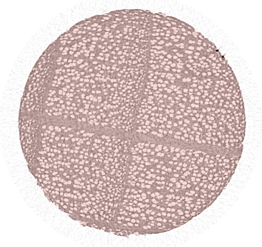
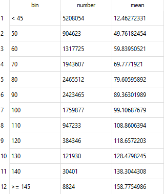
This example shows the type of output to expect. The input image, left, is a CT scan of a 4.5 mm cylindrical beech dowel, and a mask (red overlay) comprising only the pixels inside the cylinder. The bins were manually set: 10 bins of size 10, starting at 50. The third column in the resulting spreadsheet, right, shows the average greylevel of the pixels in each bin.

NOTES:

The automatic bin definition methods also use the optionally connected mask and ROI.
Empty out-of-bounds bins will not appear in the output spreadsheet. All other bins, whether empty or not, will be in the output.
If datatype is integral, and you set a bin size of 1 and the number of bins to cover the whole range of values, then the optional columns give no additional information.
If a bin has a count of 1, then the variance will be not-a-number (nan). If it is has a count of 0, then both mean and variance will be not-a-number.
The number of bins set in the Number field of the Bins port does not comprise the two potential out-of-bounds bins.
The bin setting procedure coupled with the cropping option will behave differently depending on the method used. See section Cropping and automatic bin parameters for more details.

Ports:

The ports described here are specific to the computation of the histogram. Modules using a histogram for other computations might include these ports, and more.

Bins

Bin definition. The first value, Start (noted bg₀ above), is the center greylevel of the first bin. The second value, Size is the width of the bin, noted h. Finally, Number is the number of bins, nb.

Autobin

Automatic methods to set the histogram bins. By automatic, I mean in contrast with manually setting all three parameters in the Bins port, all methods here will deduce at least one of the bin parameters.
Most of these methods are taken directly from Wikipedia (circa 2022):

Fixed number: the number of bins nb is fixed, will deduce bg₀ and h.
Integers: bin greylevels bg_i are the integers in the greylevel range. If lowest and highest greylevels are l and h, then the number of bins is floor(h)-floor(l)+1.
Square root: sets nb = √n, where n is the number of pixels (method used by Excel, for instance). Will deduce bg₀ and h.
Sturge¹: sets nb = ceiling(ln(n) + 1). Will deduce bg₀ and h.
Rice²: sets nb = ceiling(2 ³√n). Will deduce bg₀ and h.
Doane³: sets nb = 1 + ln(n) + ln(1+(|g₁|/σ_g₁)), where g₁ is the skewness of the greylevels, and σ_g₁ = √((6(n-2))/((n+1)(n+3))). It's an improvrement of the Sturge method for non-normal data. Will deduce bg₀ and h.
Scott⁴: sets h = 3.49 σ/³√n, where σ is the standard deviation of the greylevels. Will deduce bg₀ and n.
Freedman-Diaconis⁵: sets h = 2IQR/³√n, where IQR is the interquartile range. Will deduce bg₀ and n.
Optimised⁶: Iterative method that computes a cost function for each bin size, and ends up with the bin size that minimises this cost. Not yet implemented.

The Set button effectively computes and sets the bin parameters using the selected rule. Note that only the bin parameters is determined when pressing this button, the histogram is not computed.
If the Crop option is selected, will set a given percentage of pixels in the out-of-bounds bins, as given by the Crop port below.

Crop

Percentage of greylevels to crop, both on the lower and upper ends of the greylevel range.
The method is slow if the entirety of the image is used to find the exact value at which to crop, which is why a (random) subsampling is the default. The fraction of pixels to use for this subsampling (as well as the seed for the random part) can be set in the console (see setCrop_f in the Commands section).
If you want you can set the fraction to 1 to get the most accuracte cropping. But even a small fraction gets close to the percentage target. The plot below shows the error versus the fraction of pixels used (the error bars were made using 10 different seeds for the random number generator for the subsampling, see command setCrop_s below).

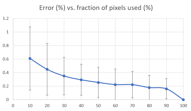
Error (%) on the percentage asked as a function of fraction of pixels used. The maximum percentage to crop is 99 %, but that would be very stupid to set it so high.

Cropping and automatic bin parameters

Because each method in the AutoBin port can determine different parameters and deduce others, their behaviour will differ when coupled with the cropping option:

For the Fixed number method, nb will remain the same, but bg₀ and h are modified.
For the others that start by setting nb, will modify it as a ratio of the cropped greylevel range to the entire greylevel range.
For the methods setting h, will adjust bg₀ and nb accordingly.
For the Integers method, will adjust bg₀ and nb so the first and last bins are the integers nearest to the greylevels asked for the cropping.

Columns

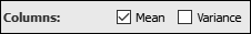
Mandatory columns are bin and number. Optional columns are mean, the average greylevel of the pixels in the bin, and variance, the greylevel variance in each bin. These can be useful for e.g. accurately determining a threshold from the histogram (see Threshold_Global).

Commands

Setting the bin parameters with some of the methods listed in the AutoBin port (and if cropping is asked for) will require sorting a sample of greylevels of the image. Sampling all values can take a long time, so the default is a subsampling. These commands determine the subsample.

`setCrop_f`

Fraction of pixels in input image (AND in the mask AND ROI, if given) to subsample in order to compute the lower and upper threshold given in the Crop port. Fraction is in the range ]0;1]. If set to 1, all greylevels are used.

`setCrop_s`

The subsampling is random, the randomness is generated with a PRNG (pseudo-random number generator), which needs a seed value. You can set the seed with this command.

`setIQR_f`

Same thing as setCrop_f, but for the IQR computation used in the Freedman-Diaconis option in the Autobin port.

`setIQR_s`

The seed for the sub-sampling for the IQR computation.

`getCrop_f, getCrop_s, getIQR_f, getIQR_s`

Retrieves the values mentioned above. Note that for the methods that require computing variance or skewness, all pixels are used.

References:

¹ Sturges, H. A. (1926). The choice of a class interval. Journal of the American Statistical Association 65-66.
² Online Statistics Education: A Multimedia Course of Study (http://onlinestatbook.com/). Project Leader: David M. Lane, Rice University (chapter 2 "Graphing Distributions", section "Histograms").
³ Doane DP (1976). Aesthetic frequency classification. American Statistician, 30: 181-183.
⁴ Scott, D.W. (1979). On optimal and data-based histograms. Biometrika 66 (3): 605-610.
⁵ Freedman, D.; Diaconis, P. (1981). On the histogram as a density estimator: L2 theory. Zeitschrift für Wahrscheinlichkeitstheorie und verwandte Gebiete 57 (4): 453-476.
⁶ Shimazaki, H.; Shinomoto, S. (2007). A method for selecting the bin size of a time histogram. Neural Computation 19 (6): 1503-1527.