List of my modules...
Module: Threshold_Global
Description:
Converts image to "black and white" with a simple global thresholding. I used quotes because it depends on the greylevels you set in the Values port, and if you set a third greylevel for the outside is a mask or ROI (region of interest) is connected.
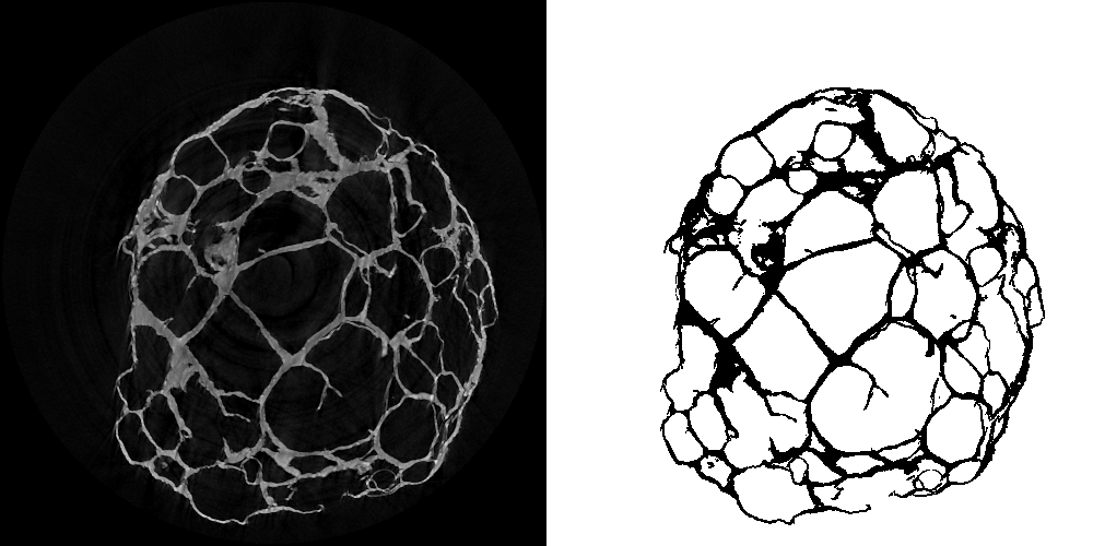
Illustration of the binarisation procedure. Original image is on the left, result on the right, in which the object is defined as black, and background as white.
Notes
- No automatic method to set the threshold was developed with an equality comparator in mind (= or ≠). More specifically, the methods were implemented with the ≥ operator (< would produce the same result, and in most cases, so will the other two ordering operators).
- If a histogram method is selected and there's a histogram connected at the input, then the module will use that histogram (provided it's valid). If not, no matter if a histogram has already been computed by the module (at the output), it will always recompute the histrogram.
Connections:
Image
[required]
The input image, of type HxUniformScalarField3.
ROI
[optional]
A Region Of Interest (ROI), defined in a HxSelectRoi. Will only count the pixels in the ROI if one is connected. A pixel is defined as in the ROI if the intersection between the ROI and the unit cube that defines the volume occupied by the pixel is non-empty.
Mask
[optional]
A mask image, defined in a class HxUniformScalarField3. Will only count the pixels if the corresponding pixel in the mask satisfies the threshold comparison defined in the appropriate ports.
Histogram
[optional]
A pre-computed histogram, defined in a class HxSpreadSheet. This can be useful if e.g. the histogram was generated on reference region or reference image, and the threshold needs to be computed from there for the connected image or the set region.
The histogram must have the same structure as that generated by the module Histogram_ (detailed here).
Ports:
Threshold

Value to compare with the pixel intensity.
Comparison
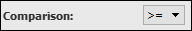
Defines how the threshold is used to define the pixels of the object.
Values

Values in the resulting image for the object and background.
Automatic choice of threshold
This part is for automatically choosing a threshold value. Hopefully I'll add more methods as I go along...
Auto
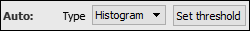
Sets the type of automatic threshold selection: none, histogram-based or iterative. Pressing the button only sets the threshold in the Threshold port (does not check the comparator in the Comparison port).
AutoHisto

Selects the type of histogram-based threshold value selection. If a histogram-based method is selected (and if no histogram is connected at the input), then additional ports will be displayed for defining the histogram. See here for details about these (Warning: port ordering is haphazard, so they can appear in the middle of the others).
Peaks
This is an implementation of the algorithm described by Sezan1, with a few customisations. The original core of the method is as follows:
- Compute Cumulative Distribution Function (CDF)
- Smooth CDF: using an averaging window of given size (an odd number).
- Subtract smoothed CDF from CDF: this is equal to the derivative of the smoothed histogram (see appendix in cited paper. And I checked, it works...). The result is called the Peak Detection Signal (PDS).
- Find peaks: in the PDS, a peak is defined by three values. The peak start is when a negative crossover is found (going from positive to negative values). The peak maximum is the following positive cross-over. The peak end is the local maximum between the start of the current peak and the start of the next one.
The paper goes on to describe a closeness criterion between two peaks so as to merge them when necessary (depends on the application). This criterion is equal to the difference between the greylevels of the end of one peak and the start of the next. The merged peak starts at the start of the first one, ends at the end of the second one, and its maximum is the biggest of the maximum of each.
Finally, the threshold value selection presented is a weighted average between the end of one peak and the start of the next.
Implementation and customisations
Intermediate data are stored in the histogram HxSpreadsheet in an additional table named Peaks.
- Histogram and CDF: starting with table Histogram, the first column, Greylevel, gives the greylevel of the center of the bin, the second column, Number, is the number of pixels in that bin (i.e. closer to that bin's center value than any other bin center value), and the third, Cumulative, is the sum of the number of pixels in that bin and the number of pixels in all preceding bins.
- Smoothed CDF: the half-size of the averaging window for the smoothing of the CDF is defined by the N/2 value set in this port. The size of the window will then be (N/2)*2+1=W (like that it's always an odd number). The cited paper does not explicitely describe what happens on the CDF border, where the averaging window only partially overlaps the CDF. It implies zero-padding, but when doing it that way, the end part of the PDS shoots out the roof, and when merging peaks in the final part of the method (i.e. finding the biggest of the maxima), it always chooses the greylevel of that last peak's maximum, which is bad. So instead of systematically dividing the sum of the PDS values in the windows by W, I divide that sum by the number of values in that window (e.g. N/2+1 when at the CDF border). That way, the subtraction of smoothed CDF from CDF will not shoot up. The smoothed CDF is in column four, Averaged.
- PDS: or the difference between the two last columns, is in the fifth column, PDS
- Peaks: the set of peaks, defined by their start, end, and maximum, are found and stored in the second table, called Peaks, in the first three columns, intelligently named Start, End, and Maximum. Note that in these columns it isn't the greylevels that are stored, but the row indices to the corresponding greylevel (starting at 0). In other words, a value of i refers to the greylevel at row i+1 in table Histogram.
- Merge peaks until two remain: the paper suggests that when a fixed number of quantisation levels is sought (in our case, we want two), then the averaging window should first be automatically adjusted before some final merging is applied with the closeness criterion. I found after a few tests that changing the averaging window size would alter the result in a bad way, more often than not. So to simplify the process, I find the two consecutive peaks that are farthest apart using that closeness criterion, and merge with the left one all peaks before it, and merge with the right one all peaks after it. The fourth column in the Peaks table, called Index, is the row number (again, starting at 0) to the maximum of that merged peak. This means that you can see where the pair farthest apart is and how the peaks were merged (all peaks with the same value have been merged). Note that this value is a row number to the Maximum column, itself a row number to the Greylevelcolumn in the first table. It's like the movie Inception, but with arrays instead of dreams.
- Find and set threshold value: contrary to the paper, I set the threshold value to the average of the greylevels of the maxima of the two final peaks.
Notes
- The N/2 value doesn't need to be huge (the default seems sufficient for typical applications).
- Even if plenty of peaks are found, the merging process seems fairly robust.
Otsu
This method is an discrete analog of Fisher's linear discriminant2, and was introduced by the namebearer Nobuyuki Otsu in a hugely cited paper3.
It finds the grey-level threshold θOtsu such that the variance between the two classes of pixels defined by that threshold is maximum. In maths it can be written as:
θOtsu = argmaxθ{∑k<θp(k)(μ0 - μ)2 + ∑k≥θp(k)(μ1 - μ)2}
Where:
- p(k) is the normalised histogram
- μ is the average grey-level
- μ0 is the average grey-level for all pixels that have a grey-level < θ
- μ1 is the average grey-level for all pixels that have a grey-level ≥ θ
Contrary to the original definition, this implementation does not necessarily compute the threshold on integer grey-levels. It uses those defined by the histogram.
Bayesian
This method supposes that the image is made up of two classes of greylevels each having a Gaussian distribution. In other words, we suppose that the histogram is a union of two Gaussians. A (normalised) Gaussian can be defined by an expected value μ and variance σ2, and is written g(x) = (1/√(2π)σ)exp(-(x-μ)2/σ2). This can also translate as the probability of observing x in such a distribution.
The idea is that a threshold value defines two groups, one containing all pixels with a strictly smaller greylevel, and with greater or equal greylevel. From each, the mean and variance are computed (μ0, σ0, μ1, σ1) and define the Gaussian distribution for each group. In this framework, the optimal threshold θ would have an equal probability of belonging to either group, i.e. g0(θ) = g1(θ).
In practice, we test only the values defined in the histogram, and we won't find a threshold θ such that g0(θ) is perfectly equal to g1(θ). What is done instead is that for each threshold candidate x, the two Gaussians are determined and (i.e. the means and variances are computed), and g0(x) and g1(x) are calculated. We then compute the ratio of the largest by the smallest: max(g0(x), g1(x))/min(g0(x), g1(x)). From all the candidates defined by the histogram bins, we choose the one with the ratio closest to 1 as θ.
Notes
- Creates columns Prob_0 and Prob_1 in the resulting spreadsheets, containing g0(x) and g1(x). Is the verbose command is used, also created columns containing the means and variances.
- I didn't find any references describing this method, so I did it myself. If I got it wrong, please let me know.
AutoIter

Selects the type of iterative threshold value selection, when the relevant option is chosen in the Auto port.
Isodata
Widely used in 2D medical image processing, this is a iterative clustering algorithm that sets the threshold as the average of the means of the grey-levels of the two clusters4:
- Set arbitrary initial threshold th, here as the middle of the grey-level range.
- Compute means μ0 and μ1, the mean grey-levels of pixels belonging to each group, defined by the threshold th and comparator set in the Comparison port.
- Set new threshold th' = (μ0 + μ1)/2, if th'≠th then set th←th' and repeat.
Note that sometimes the (light) pixels of the object have a higher variance than the (dark) background, and using this method on the logarithm of the image rather than the image itself gives better results.
Porosity
Finds the threshold such that the percentage of pixels with a greylevel stricly lower than the threshold best approaches the percentage given.
Note on the iterative methods
On very large images, it takes a long time to iterate over all the pixels, so these methods are first computed on 1 % of the pixels (random sampling), and when it converges it does the same on 2 % of the pixels, and so on (doubling every time) until 100 %. Quite often the threshold found with 1 % of the pixels will stay there until the end of the process.
Commands:
Additional options can be accessed when typing in the console Binarise COMMAND_NAME.
verbose
Displays timing information after the computation. Retype to hide info.
create
Runs the computation. Returns the name of the output, so it can be used in a script, such as set RESULT [Binarise create].
Scripting:
Typical use in a TCL script would look like so:
	set B [create Binarise]
	$B Image connect $INPUT_IMAGE; $B fire
#	$B Threshold setValue $THRESHOLD; $B Comparison setValue 3
	$B Auto setValue 2; $B fire
	$B Iter_Method setValue 3 1; $B fire
	set OUTPUT_IMAGE [$B create]
References:
1 Sezan, M. (1990). A peak detection algorithm and its application to histogram-based image data reduction, Computer Vision, Graphics, & Image Processing 49: 36-51.
2 Fisher, R. A. (1936). The Use of Multiple Measurements in Taxonomic Problems. Annals of Eugenics 7 (2): 179-188.
3 Otsu, N. (1979). A threshold selection method from gray-level histograms. IEEE transactions on systems, man, and cybernetics SMC-9 (1): 62-66.
4 Ridler, T. W.; Calvard, S. (1978). Picture Thresholding Using an Iterative Selection Method. IEEE transactions on systems, man, and cybernetics SMC-8 (8): 630-632.