Module: Skeleton_Process

Description:

Post-processing of the skeleton to determine element (or pore, or cluster) positions, for instance by merging neighbouring nodes (i.e. setting the same label) under specific conditions, or creating new ones in previously unidentified openings.
The idea behind this module is that the input skeleton graph contains the topological information of the original shape, and for a representative view of the structure we feel the need to add in geometrical information, as simply saying that branch intersections in the graph represent an element is oversimplifying things¹.

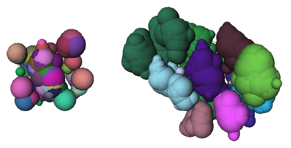
Left: Portion of the result of the conversion of a skeleton to a graph (using Skeleton_Image_To_Graph). Right: processing of the graph to relabel nodes belonging to the same opening. More of the graph is displayed here because adjacent nodes with the same labels are drawn (using Draw_Skeleton).

NOTES:

• In the rest of this document, I use the following notations and definitions. nX is node X, vX is its associated value. These two represent a maximal ball BX centered on nX with radius vX that can be placed in the original structure. V(BX) is the volume of ball BX, and Vo(BX,BY) is the volume of the intersection between balls BX and BY. ClX is cluster X, i.e. a set of nodes that have the same label, and thus represent the same element in the structure. Finally, d(nX,nY) is the Euclidean distance between node X and node Y.
• All the methods presented below are independent, sequential, and done in that order if several are selected.

Connections:

Skeleton

[required]
The skeleton, of type HxSkeleton.

Ports:

Merge


Merges connected nodes under different conditions. We mean by merging assigning the same label, not actually modifying the graph structure. The first option checks for an overlap between balls, and the second option looks at the points along the edges connecting two nodes of different clusters, and if no constriction (or bottleneck) is found, then they are merged.

Overlap_Measure


Defines how the mentioned overlap is measured. If we consider nodes n1 and n2, if f(n1,n2) < x, then they are merged. The functions f() and values x are described below. Note that there are plenty of different conditions in the literature (see section 2.5.1 in the reference), and you can choose to test a few here:
• Maximum: d(n1, n2) - max(v1,v2) < x. The value x can be viewed as an error margin. If it equals 0, the condition is equivalent to checking if one node is contained in the other maximal ball.
• Sum: d(n1, n2) - (v1+v2) < x. Again, x is an error margin, and if 0 it means that the maximal balls touch.
• Volume ratio: Vo(B1,B2)/min(V(B1),V(B2)) > x. This time x is a ratio between 0 and 1. This time we're looking at the volume of the intersection of the two balls, and the ratio with the volume of the smallest one. What this means is that if more than a fraction x of the volume of the smallest ball is contained in the other, then they are merged.

Error_Margin


Defines the value of x for the Overlapping merging, if the overlap measure chosen is either Maximum or Sum.

Overlap_Threshold


Defines the value of x for the last overlap measure type, Volume ratio. Compared to the other overlap measures, it is defined in a separate port because it's a bounded value (between 0 and 1), and merging is applied when greater than this value, not less.

Constriction_Delta


If the No constriction merging is selected in the Merge port, this port specifies a delta x with which to define if a constriction was found or not. If we define vc as the smallest value found along the edge (n1, n2), then we say that there is a constriction if vc < min(v1,v2) - x, and merge if this is not the case. You can imagine the edge as a tube connecting B1 and B2, then the tube radius must shrink of at least x before going from one ball to the other for there to be a constriction.

Absorb


Small clusters are absorbed into the closest connected big cluster (we say cluster here to mean the set of nodes that have the same label). We say a cluster is small if all nodes of that cluster have an small associated value (therefore it should be absorbed), otherwise it is defined as a big cluster. In essence the result of an absorption is the same as a merging, two labels become one. But there are two main differences. Firstly, in a merging we're looking at node pairs independently, whereas here we're treating the cluster as a whole (e.g. to define whether it's big or small, or how close it is to another). And secondly, contrary to the merging methods we're defining an order relation in this case, defining one cluster as small and the other as big and absorbing the small one (you can argue that we make use of the min() function in some of the previous merging methods, effectively also defining an order relation, but that's not really true, as it's just used to define a measure, not to provide an order relation).

This absorption process uses a distance-ordered propagation-type absorption algorithm, broadly described by the following steps:

1. Find all pairs {Cls, Clb} of neighbouring clusters such that Cls is small and Clb is the closest big cluster.
2. Sort and store all these pairs according to distance.
3. Extract the closest {Cls, Clb} pair, and merge.
4. Look at the clusters neighbouring Cls. Find the one(s), we'll call Cl', that are not neighbour to Clb and that are to be absorbed.
5. Check the distance between Cl' (if exists) and Clb, called d'. Two cases: either Cl' is already part of a stored pair, in which case, if d' is smaller than the one already stored, update accordingly (i.e. remove pair containing Cl', and replace with pair {Cl',Clb} with distance d'). Otherwise, Cl' was not yet stored (not direct neighbour to a big cluster), so add in the {Cl', Clb} pair.
6. Repeat from step 3 until no more pairs are stored.
NOTES:
• The distance between clusters Cl1 and Cl2 is defined as the smallest distance between two nodes n1 and n2 respectively belonging to Cl1 and Cl2.
• The distance between nodes n1 and n2 is defined as follows. If v1+v2 < d(n1,n2), i.e. if the balls don't touch, then the distance equals d(n1,n2) - (v1+v2). Otherwise, the distance equals -Vo(B1,B2)/V(min(B1,B2)). This value is negative so that the more the overlap ratio, the smaller the distance measure (i.e. the higher the absorption priority), and it garantees that overlapping clusters will always be processed before non-overlapping ones.
• If a small cluster is not connected to any big cluster, then it won't be absorbed. As a corollary, if several small clusters are interconnected, they won't be merged together if none are connected to a big cluster.

Small_Threshold


For the absorption process described above, a cluster is defined as small if for all nodes nX of that cluster, vX < x, where x is defined by this port. If at least one node nX is such that vX ≥ x, then it is considered a big cluster.

Insert


Inserts new nodes (with a new label) on certain edges. The first option checks whether there are two or more constrictions along an edge and if the local maxima in between each pair has a sufficient dynamic, and if so new nodes are created between those constrictions. The details of this condition is described in the Dynamic port description.

The second option supposes boundary conditions, and creates new nodes on the edges that traverse the bounding box, at the position where the intersection occurs.

Dynamic


This process supposes that several elements are connected to each other in a chain, as in the following figure:

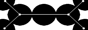
where the original structure is in black and the skeleton graph is superimposed in white. Obviously we'd like to have a new node inserted in the center of that edge. The way this is done is by finding all the local minima along an edge, and if for two such minima, called m1 and m2 there is a local maximum M in between such that M-max(m1,m2) > Dyn, where Dyn is the dynamic defined by this port, then a new node is inserted, at the position M and with a value equal to this local maximum.

Options


This option, Relabel, modifies the labels of all the clusters so that all labels have consecutive non-zero values starting at 1. This option used to be by default for a stupid practical programming reason (although it still is useful for subsequent processing), but not modifying the labels has the advantage of being able to better visualise how the labels have been changed after the processing.

Action button


Push the button to start the computation.

Commands:

Additional options can be accessed when typing in the console Skeleton_Process COMMAND_NAME. Typing the command again usually reverts back to original settings.

verbose

Displays timing information after the computation. Retype to hide info.

create

Runs the computation. Returns the name of the output, so it can be used in a script, such as set RESULT [Skeleton_Process create].

tryMergeEveryPair

For the node merging process, the default is to try to merge only the nodes of the edges of the graph, but sometimes two nodes can be merged even though they are connected through a third node (i.e. no edge directly linking them). In this case, this command tells the module to try to merge every node pair in the graph, whether or not they share an edge.

References:

¹ E. Plougonven, Link between the microstructure of porous materials and their permeability, PhD thesis, Bordeaux, 2009.