List of my modules...
Module: Distance_Histogram
Description:
Given an image I and a map M of same size (e.g. like a distance map), computes statistics on subsets of pixels of the image, thoses subsets defined by the map. Outputs a spreasheet with various values as a function of those from the map.
The subsets are defined by the map as bins in a histogram. The first bin starts at a user-defined value start (see ports below), for instance if in your map you want to consider all pixels marked with a non-zero value, then start = 1. The bin size is the user-defined value step, so that the first subset of pixels will be those that have a value in the map between start and step. The ith subset, Gi is the subset of pixels p such that start + i.step ≤ M(p) < start + (i+1).step.
Given that μi = (1/N)∑(xi-μ)k is the kth central moment of the values xi of the pixels in that subset, the columns in the spreadsheet are:
- Value: The smallest value of the bin, start + i.step
- Number: |Gi|, the number of pixels in that group
- Mean: <I(p)>, p ∈ Gi, the average greylevel in the image for the pixels of that group
- Variance: μ2=σ2 the square of the standard deviation
- Skew: μ3/σ3
- Kurtosis: μ4/σ4
There is an option for cumulative statistics, in which case a new table in the spreadsheet is created with the same columns, but the subsets add up, meaning that the ith subset Gci contains the pixels p such that start ≤ M(p) < start + (i+1).step.
Examples below:
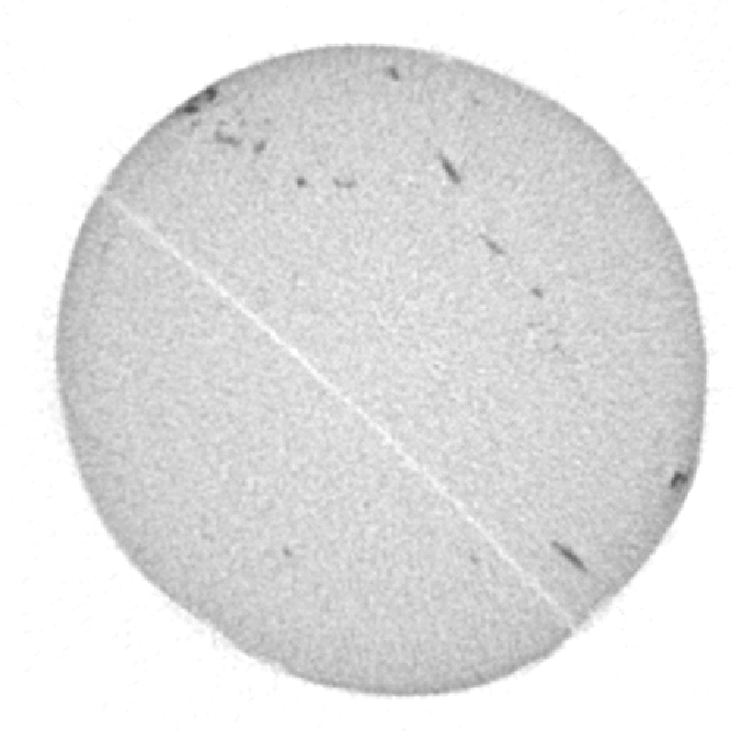
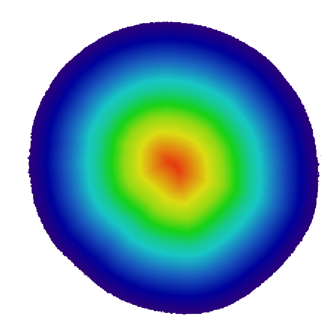
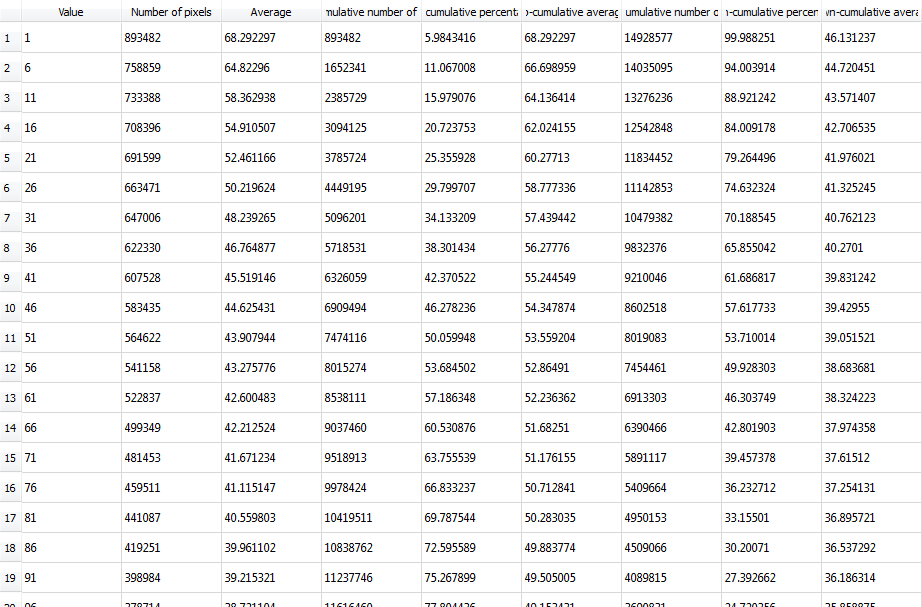
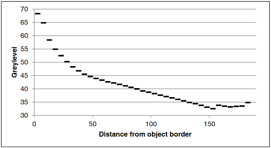
Top left: input image, a tomographic cross-section of a cylindrical clay sample, with some beam-hardening artefact. Top right: a colored distance map of the interior of the sample, values representing the distance from the outside (white is zero or unassigned, blue to red is 1 to 190). Bottom left: resulting spreadsheet when image and map are those above, with values computed with increments of 5, starting at 1. The bottom right shows the average greylevel from the input image (third column) as a function of distance from the border (first column), which allows to see the amount of beam-hardening there is (supposing the sample is homogeneous, obviously).
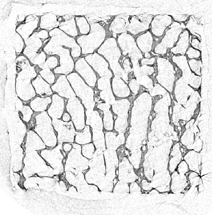
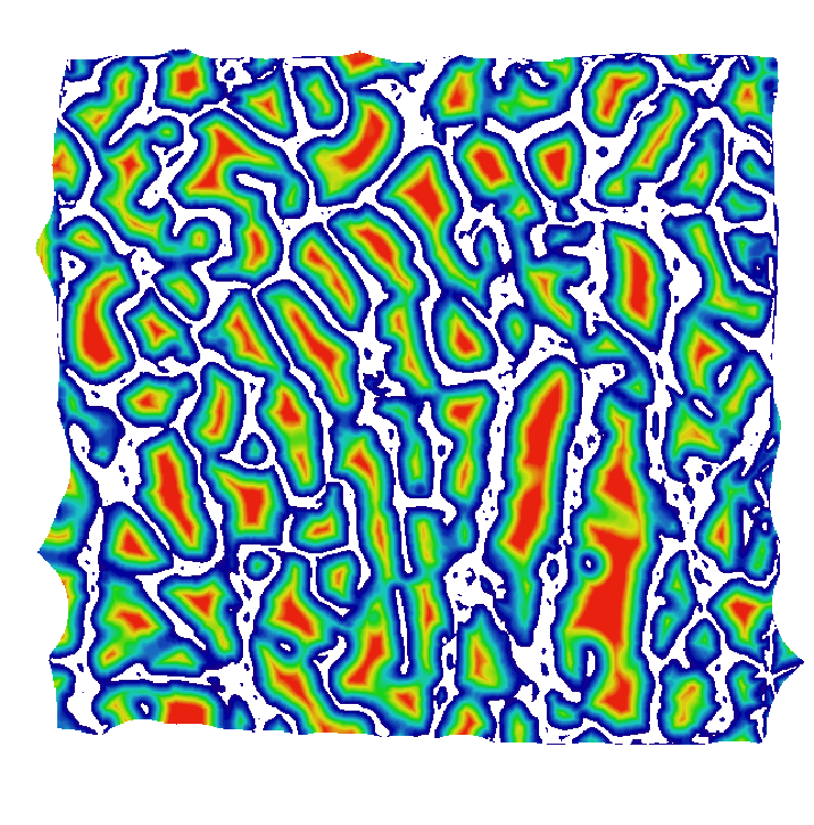
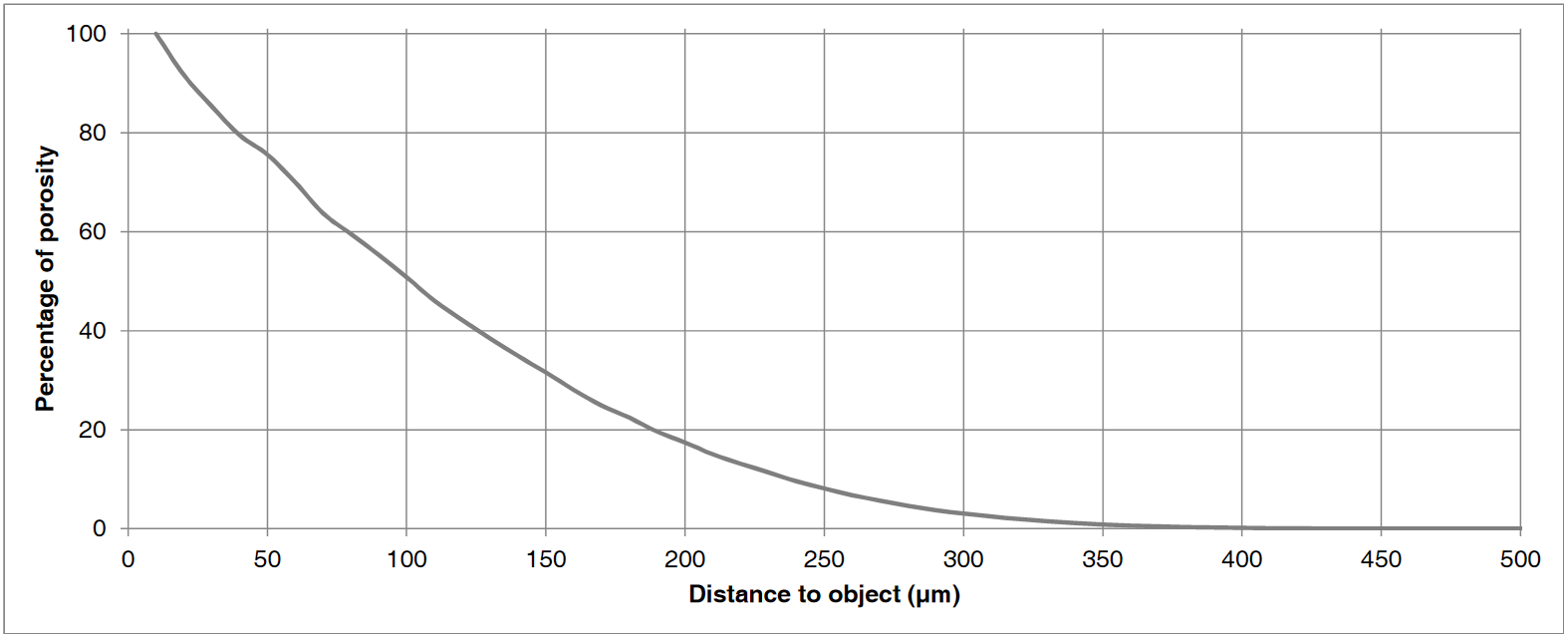
Top left: input image, a tomographic cross-section of a bone sample. Top right: a colored distance map of the interior of the sample, values representing the distance (in microns) from the bone (white is zero or unassigned, blue to red is 1 to 300). Bottom is the result when input image and map are both set to the distance from the bone: it plots the percentage of pixels from the porosity that are at least at a given distance from the bone, i.e. seventh versus first column.
Notes
- The non-cumulative normal statistics cannot be unticked because they still need to be calculated for the cumulative ones (given the one-pass algorithm I've implemented [1]), might as well put them in the spreadsheet.
Connections:
Image
[required]
The input image, of type HxUniformScalarField3.
Map
[required]
The input map, of type HxUniformScalarField3 and of same size.
Ports:
Start_at

Allows to consider only the pixels p such that M(p) ≥ start
Step

Size of each interval.
Tables
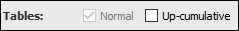
Can add a table with cumulative values. Normal table is always there (see notes).
Now
Push this button to start the computation.
Commands:
Additional options can be accessed when typing in the console Distance_Histogram COMMAND_NAME.
verbose
Displays timing information after the computation. Retype to hide info.
create
Runs the computation. Returns the name of the output, so it can be used in a script, such as set RESULT [Distance_Histogram create].
References:
1 Pébay, P. (2008). Formulas for Robust, One-Pass Parallel Computation of Covariances and Arbitrary-Order Statistical Moments, Sandia National Laboratories.